From autoplot.org

Audience: Science Community

Purpose: Autoplot is described in this introductory guide. This includes an initial section on plotting data in Autoplot, and then later sections introduce scripting and introducing new data sources into Autoplot.

Contents Introduction Data is Identified with URIs Browsing the Data More Mouse Actions .vap files Bookmarks File Cache layout tab metadata tab Autoplot Plots Data From Many Sources Overriding the Data Source Type Launching Autoplot Power Users and Admins Aggregation Data can be output in many ways There are many hidden features Das2 Graphics Library Autoplot DOM Java BeansBinding Autoplot Data Handling Scripting Architecture

1. Introduction

1.1. Data is Identified with URIs

Autoplot (http://www.autoplot.org) plots data from many different sources using an interface that is familiar and simple.

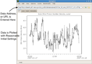
Data address, or URI, is entered in an address bar, and the data is plotted with reasonable initial settings.

Data URIs are often URLs, such as the location of an CDF file, plus additional parameters that identify a plottable parameter. For ASCII tables, the file resource is identified, and the URI parameters may configure the parser used to read the data. Here are some example URIs:

 http://cdaweb.gsfc.nasa.gov/istp_public/data/ace/swe/2008/ac_k0_swe_20080816_v01.cdf?Np
 ftp://nssdcftp.gsfc.nasa.gov/spacecraft_data/omni/omni2_1977.dat?time=field0&timeFormat=$Y+$j+$H&column=field8&fill=999.9

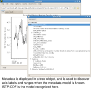
Metadata is displayed in a tree widget, and is used to discover axis labels and ranges when the metadata model is known.

Browse to a file resource using file system completions to list the remote folder. Clicking on the folder icon triggers completion, which is a list of options that build the URI. Autoplot is able to browse HTTP and FTP filesystems as if they were local.

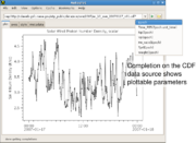
Data Sources provide completion engines to configure the URI. Completion on the (NASA/SPDF) CDF data source shows plottable parameters. Completion is triggered by tapping control and space in the address bar. When the URI is incomplete, for example if just the name of a CDF file is entered without the parameter name, completion is triggered to guide the user.

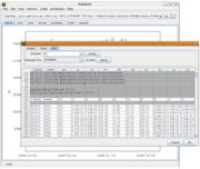
Some data sources have graphical user interfaces for creating URIs. For example, clicking the folder icon for an ASCII text file displays the data in a table, indicating how the data will be parsed. GUI components allow the parsing to be configured. When the file is parsed properly, the ascii file URI is updated and the file is parsed completely for plotting.

1.2. Browsing the Data

Browsing the data is fast and intuitive.

zooming. To zoom in, drag out a range with the left mouse button. The mouse wheel works as in Google maps: press the mouse wheel and drag to pan the axis. Spin the mouse wheel to zoom in and out. Similar gestures on the x or y axis will adjust just the one axis.

undo/redo. Control-Z will undo the last operation performed, and control-Y will redo the operation. These actions are found under the "Edit" menu of the menu bar, as well as the option to undo many operations at once.

scanning. At the ends of the x-axis are hidden "scan previous" and "scan next" buttons. These are useful for scanning through a long time series dataset. Note when control is pressed while the mouse wheel is spun, the axis will pan instead of zooming.

Right-click on an axis to adjust its properties.

Right-click on a plot, and select "context overview." This creates a copy of the plot with the same data at the original zoom level. A "connector" indicates the position of the top plot on the overview plot.

1.2.1. More Mouse Actions

Additional "mouse module" actions are available by right-clicking on the plot. For example, you can draw a box around points to display data in a popup with "Display Data," measure the distance between two points with "Length," or read the mouse position with "Crosshair Digitizer." These mouse actions are extensible, and scripts may add additional functionality for interacting with data.

1.3. .vap files

/what is a .vap file /

1.4. Bookmarks

/Section on bookmarking datasets and .vap files/

1.5. File Cache

/how das2 filesystems download data and file cache manager /

1.6. layout tab

/layout tab use/

1.7. metadata tab

/explain the nodes of the tree/

1.8. Autoplot Plots Data From Many Sources

Autoplot plug-ins allow it to access many different forms of data. Plug-ins adapt file formats, and also interfaces like OpenDAP. For example, the Java NetCDF code is adapted for Autoplot so that NetCDF files can be read in. Here are a few examples with the file extensions:

• Ascii tables (.dat, .txt, .csv) Data in flat ascii tables. By default a delimiter is identified and newlines separate the fields.
• Binary tables (.bin) Data in flat binary tables. Parameters configure record length, data types, endianess, etc.
• Excel speadsheets (.xls) Data is read via the Apache POI library.
• CDF files. (.cdf) SPDF CDF files are binary files with embedded metadata used commonly in Space Physics.
• CEF files. (.cef) Cluster Exchange Format is used on the Cluster mission.
• NetCDF files. (.nc, .ncml) Binary files with metadata used commonly in Atmospheric and Oceanic Physics.
• OpenDAP (.dds) HTTP-based servers for transmitting data and metadata used commonly in Atmospheric and Oceanic Physics, but NASA/SPDF provides a server as well.
• Fits files. Images used commonly in Astronomy.
• Wav files. (.wav) Sound files are read in, mostly because the files are familiar and contain both data and metadata.
• Image files. (.png, .jpg) Images are read in, again because the files are familiar. But occasionally it's useful for digitizing applications.
• TSDS Server. (.tsds) Virbo Time Series data server has a custom plug-in for getting data at many time scales.
• QStreams (.qds) is a serialized version of the Autoplot internal data model, useful for exchanging data, caching, etc.

To see a list of the active plug-ins, enter "about:plugins" in the address bar.

1.8.1. Overriding the Data Source Type

Often you need to explicitly set the data source type, for example, with a binary file with a .dat extension. In this case you can fully-qualify the URI with the extension:

 vap+bin:file:///home/user/data/foo.dat

1.9. Launching Autoplot

The production version of Autoplot is launched from a link at the top of http://www.autoplot.org.

Autoplot is released using Sun Microsystems' Java Webstart and runs on Java 1.5. When webstart is properly configured, Autoplot is launched by clicking a link on a web site. Most desktops have Java installed already and can run webstart applications. The production version of Autoplot is linked at the top of www.autoplot.org.

Java can be downloaded freely from Sun (or Apple), and instructions for configuring webstart can be found at www.autoplot.org.

Development versions of Autoplot are distributed on the Autoplot site. These releases help to prove new features and provide quick access to bugfixes without the rigor of a production-quality release.

Note that Autoplot is also supported as a single executable jar file, an applet, and as a servlet.

2. Power Users and Admins

Autoplot is different from other plotting tools in a number of ways:

• simple, general-purpose interface increases acceptance and broadens utility
• Java Webstart makes installation and maintenence trivial
• remote filesystem layer plus aggregation templates provide excellent browsing using a simple server
• handles data at many levels of abstraction, from array of numbers to timeseries with physical units
• all data is converted to standard, uniform model
• anti-aliased fonts and graphics improves ledgibility and appearance
• highly interactive graphics components
• extensible plug-in data sources
• plug-ins output digital data to Excel, CDF, many others to come
• Jython scripting allows derivation of new datasets, complex applications, and programmatic control
• separation of Model and Controller code from View allows for use on the server-side as well as client-side
• open-source, and building procedure documented from SVN checkout to invocation

In this section we explore some of the more advanced features of Autoplot.

2.1. Aggregation

You can use file name templates to aggregate multiple files into a long time series. MenuBar->Bookmarks->Make Aggregation can do this automatically.

2.2. Data can be output in many ways

• Render to SVG, PNG, and PDF
• Save Autoplot configuration to .vap file
• Copy and Paste image into email or PowerPoint
• Export Data to ASCII table, Excel Spreadsheet, CDF, Binary table

2.3. There are many hidden features

• The menu bar contains many features, such as exporting data, bookmarks, and local file cache management.
• The Tabs "Canvas," "Axis," "Metadata," etc, undock so that the panels can be viewed side-by-side.

2.4. Das2 Graphics Library

Das2 is the graphics library used for rendering and interacting with the plots. The library provides many of the useful features found in Autoplot, such as:

• Anti-aliased graphics rendered with the Java 2D library.
• Rendering directly to SVG, PDF, and PNG.
• Mouse Modules. Mouse Modules handle the low-level mouse events to create useful science actions such as horizontal, vertical, and angle data slicing. Many modules such as length, display selected data, and crosshair digitizer are selected by right-clicking on the component.
• Property Editors. Many graph components and the DOM can be edited by right-click, edit properties. This component edits any Java Bean, quering the object for its adjustable properties. Also this can edit multiple nodes of the same type simultaneously. For example, select a few panels, then edit panels.
• Tear Off Tabs. The application comes up as a deck of tabs containing different component groups: plot, style, axes, etc. Any of these can be undocked into a separate pane for side-by-side viewing. Also the "slide right" feature has been added recently, which creates a new window that is stuck to the original pane.
• Renderers. The data is rendered with das2 renderer objects. Editing the renderer directly allows fine control of rendering.

More information about it is available at http://www.das2.org.

2.5. Autoplot DOM

The DOM is a tree of objects that represent the application state. This tree is used to create configuration files (.vap files), store information for undo/redo, and describe the unlimited number of configurations for the application. For example, application.plots is the array of all the plots on the canvas. application.panels are the panels that render the data URIs onto the plots. You can look at the DOM (and edit any property of the application) with Edit->Edit DOM on the menu bar.

Note many of the nodes of the DOM tree have a "controller" node below them. The controller object manages the node, and properties under it will not part of the application state and will not be saved to .vap files. Note that by way of the controller, you can drill down into the das2 objects that are used to implement the application.

2.6. Java BeansBinding

Java BeansBinding is a relatively new java technology. It makes it easy to connect properties of objects together, and is used throughout Autoplot to make a flexible application. For example, you can add a binding that forces the y-axes of all the plots to have the same range. This is done graphically by right-clicking on a y-axis, select "Add Binding..." then "Bind to Plot Above". As new plots are plotted, Autoplot may guess if the plot should be automatically added to the application's timeRange property so all time axes display the same time. Bindings can be created programmatically from the console with the "bind" command.

2.7. Autoplot Data Handling

Autoplot uses Data Source Plug-ins to access new data sources. The plug-ins standardize the data and metadata, but also provide the schema for creating valid URIs. Data sources are registered by extension and optionally mime-type. A URI can explicitly request a data source by using "vap+ext:" as the uri scheme. Some plug-ins also provide formatting, adding another option to the export data dialog. You can look at the list of loaded plug-ins by entering "about:plugins" in the address bar.

"QDataset" is the working name for the internal data model. It borrows good ideas from NetCDF, CDF, and CEF. It uses a thin syntax layer and semmantics to achieve abstraction. QDataSets can be serialized to a "QStream" without any information loss.

2.8. Scripting

Jython is the Python language in Java. Autoplot presents a programming interface so that Jython can be used to programmatically control Autoplot. QDataSets can be used with operator overloading to form an expressive language with rich operators, such as unit-aware addition, slicing and subsetting.

New datasets can be derived using Jython scripts. There are example scripts on the Autoplot website.

Note, Autoplot can also provide data to IDL and Matlab. This is documented on the Autoplot website.

Jython scripting introduces flexibility. For example, two parameters are read in and plotted against one another. Scripting is also used for batch plotting of data, adding features, and other tasks.

The Script panel is enabled using Options->Enable Feature->Script Panel.

2.9. Architecture

Model-View-Controller Architecture makes Autoplot well-suited for server side applications as well. An example servlet is provided that shows how Autoplot and Tomcat make a high-performance graphics server.